library(tidyverse)
library(here)
library(rio)

linelist <- import(here("processed_data", "combined_linelist.rds"), trust = TRUE) %>%
  mutate(
    age_cat = fct_relevel(age_cat, "Under 18", "18-29", "30-39", "40-49",
                          "50-59", "60-69", "70-79", "80+", "Unknown"),
    outcome = fct_relevel(outcome, "Recover", "Death", "Unknown")
)Session 6: Plotting Basics with ggplot2
The grammar of graphics, histograms, mapping vs setting, scatter plots, box plots, labels, and themes
NoteIn this session you will learn to
- Explain the three parts every ggplot needs: data, aesthetics (
aes()), and a geometry (geom_) - Make histograms, scatter plots, and box plots
- Tell the difference between mapping a variable to color and setting a fixed color
- Add titles, axis labels, and a theme
Before you start: open the workshop folder in Positron (File → Open Folder…) and open student_scripts/Session 6 - Plotting Basics_STUDENT.R. This session starts from combined_linelist.rds and measles_final.rds, the files you saved in Session 3. If you missed it, ready-made copies are already in the processed_data/ folder.
Where this session fits. Today is about one step, Visualize (highlighted): turning the clean data into plots that show its patterns. Session 7 continues with more kinds of plots and with saving them to files.
- Import
- Inspect
- Clean
- Combine
- Reshape
- Summarize
- Visualize
- Save and share
- Automate
Part 1: Set up
👀 Follow along 1.1 — Load tidyverse, here, and rio; import combined_linelist.rds as linelist, and put age_cat and outcome in order with fct_relevel() (same as Session 5).
The factor order from Session 5 isn’t saved in the file, so we set it again right after importing.
Part 2: The grammar of graphics
Every ggplot is built from the same parts, added together with +:
| Part | Function | Question it answers |
|---|---|---|
| Data | ggplot(data = ...) |
Which data frame? |
| Aesthetics | aes() |
Which columns go on x, y, color, fill, …? |
| Geometry | geom_...() |
What shape: bars, points, boxes, lines? |
| Labels | labs() |
Title and axis names |
| Theme | theme_...() |
The overall look |
Build it up one piece at a time, and run the code after every + so you can see what each layer adds:
👀 Follow along 2.1 — Build a plot in three steps: 1. ggplot(data = linelist), 2. add aes(x = age_years), 3. add geom_histogram() (the next three code blocks).
# 1. Data only: an empty canvas
ggplot(data = linelist)
# 2. Add aesthetics: the axes appear, but nothing is drawn yet
ggplot(data = linelist, mapping = aes(x = age_years))
# 3. Add a geometry: now we have a plot
ggplot(data = linelist, mapping = aes(x = age_years)) +
  geom_histogram()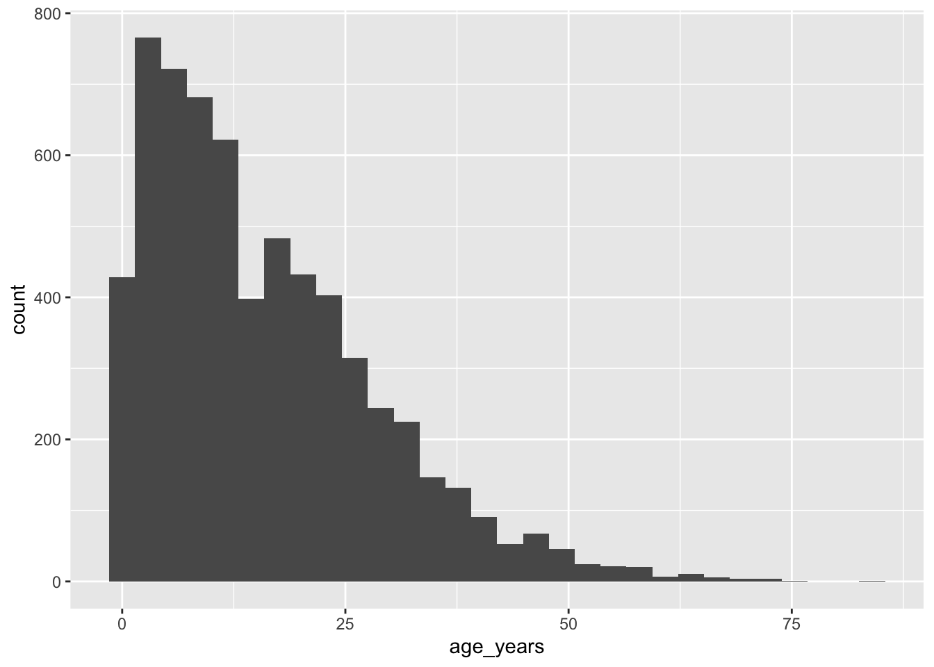
Important
+ not %>%
Layers of a ggplot are joined with +. Using %>% between ggplot layers is the most common beginner error. Like the pipe, + goes at the end of a line, not the start of the next one.
Important✏️ TRY IT 2 (2 min): build a plot in three steps
Build a histogram of measles temp_c in the same three steps: data, then aes(), then geom_histogram().
✅ Check: step 2 shows an empty plot with temperatures on the x-axis
NoteShow solution
ggplot(data = measles)
ggplot(data = measles, mapping = aes(x = temp_c))
ggplot(data = measles, mapping = aes(x = temp_c)) +
  geom_histogram()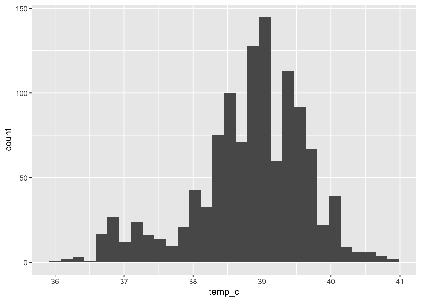
Step 1 is a blank canvas, step 2 adds the temperature axis, and only step 3 (the geometry) draws the bars.
Part 3: Histograms
A histogram shows the distribution of one number: the values are grouped into ranges (“bins”), and each bar’s height is how many values fall in that range.
R warned us above that it picked 30 bins. Choose the bin width yourself:
👀 Follow along 3.1 — Age histogram with binwidth = 5 (then try 1 and 10).
ggplot(data = linelist, mapping = aes(x = age_years)) +
  geom_histogram(binwidth = 5)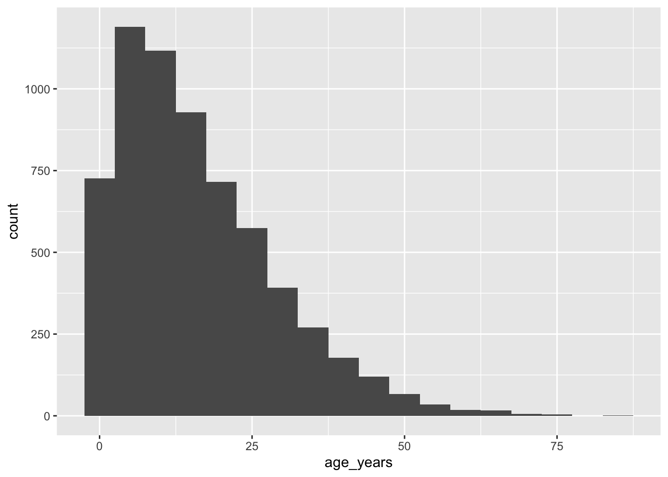
Each bar is now 5 years wide. Try binwidth = 1 and binwidth = 10 — what changes?
Fixed colors
Inside geom_histogram(), fill is the inside color and color is the outline. A white outline separates the bars.
👀 Follow along 3.2 — Add fill = "#2a78d6" and color = "white".
ggplot(data = linelist, mapping = aes(x = age_years)) +
  geom_histogram(binwidth = 5, fill = "#2a78d6", color = "white")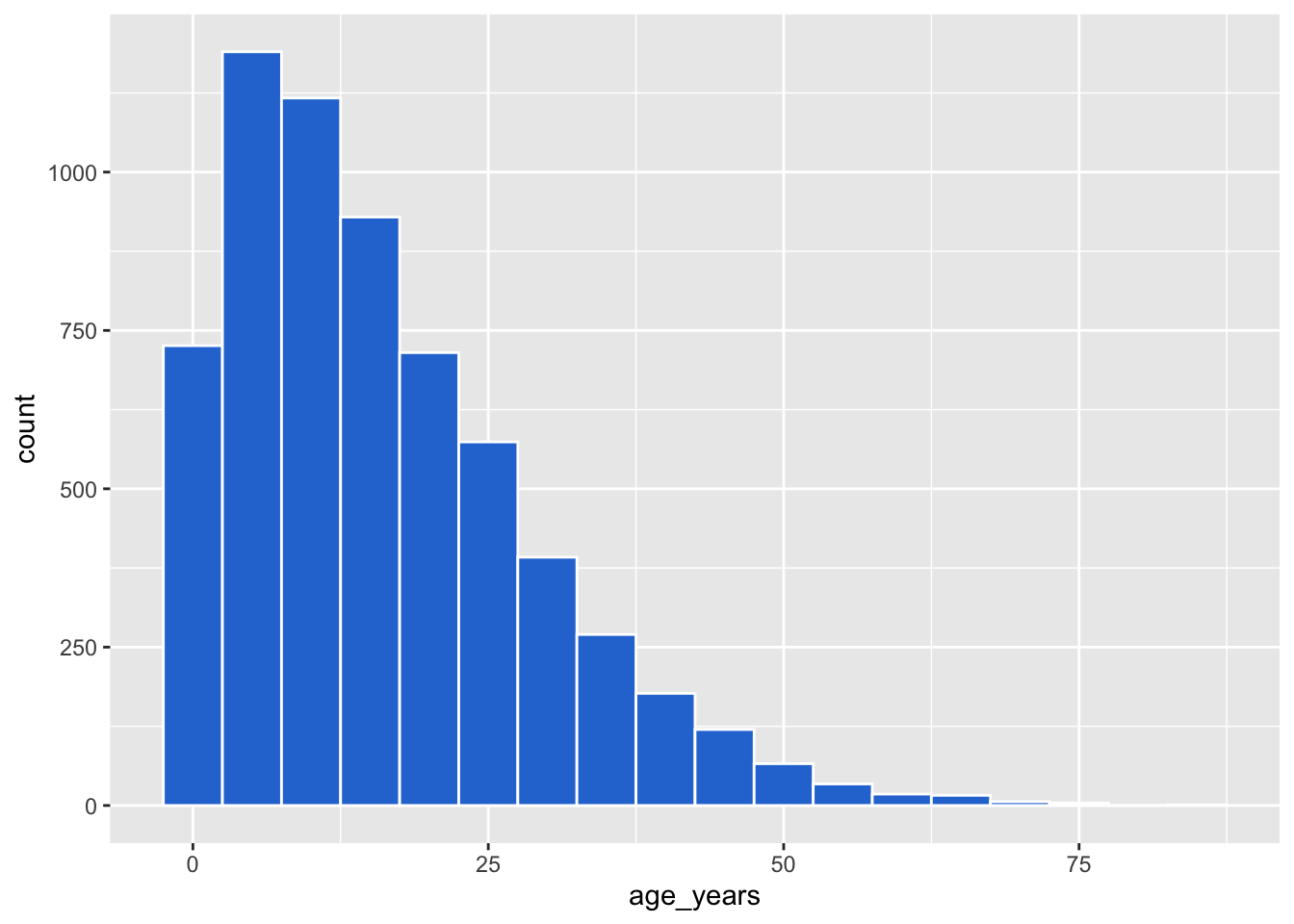
NoteColors in R
Use a name ("steelblue", "gray50") or a hex code ("#2a78d6"). Run colors() to see all 657 named colors.
Important✏️ TRY IT 3 (3 min): measles ages
Make a histogram of measles age_years with binwidth = 1, a fill color, and a white outline. Which age has the most cases?
✅ Check: the tallest bar is at age 2 (about 100 cases). The warning about “removed rows” is the 29 missing ages: that’s fine.
NoteShow solution
ggplot(data = measles, mapping = aes(x = age_years)) +
  geom_histogram(binwidth = 1, fill = "#2a78d6", color = "white")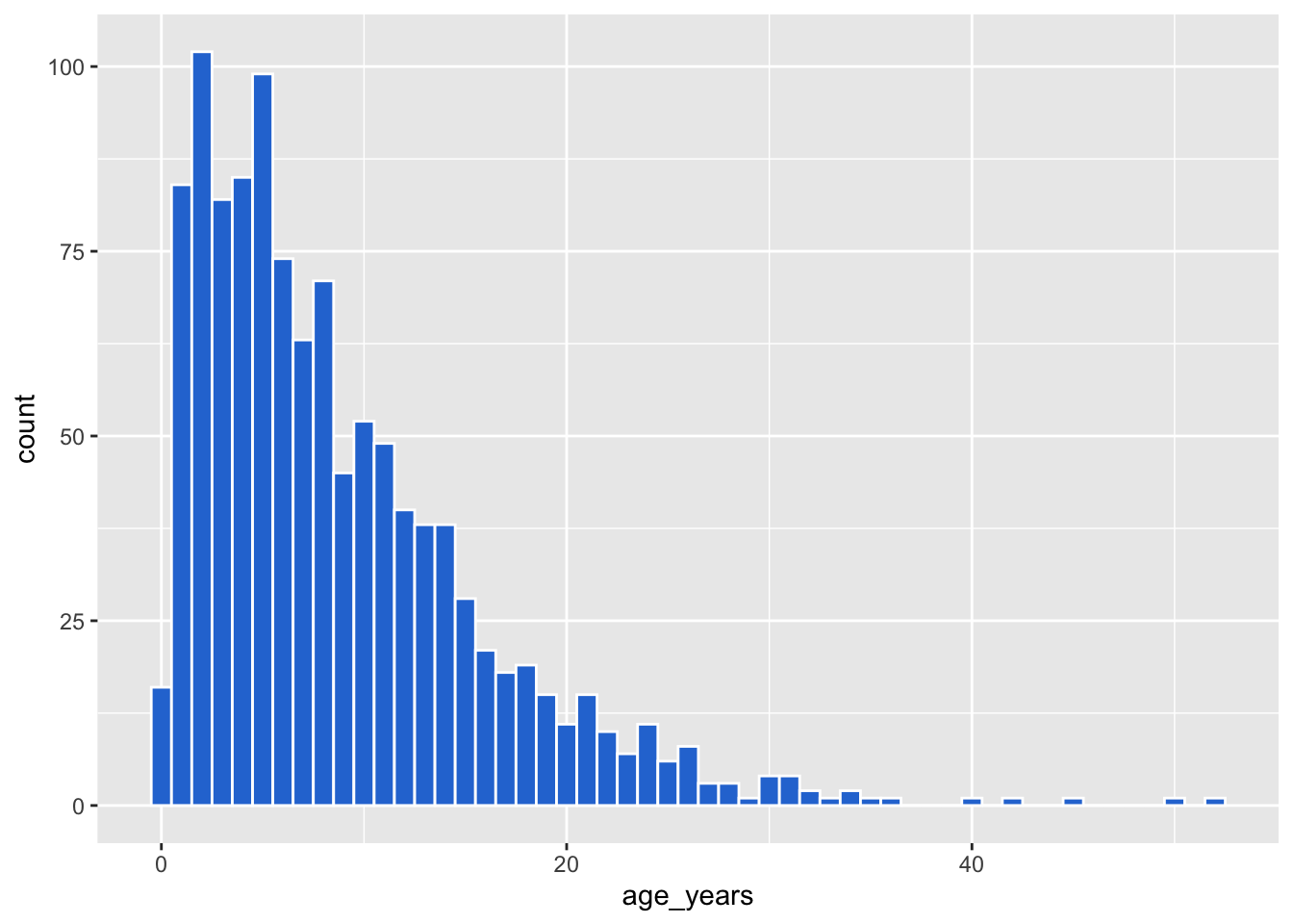
The tallest bar is age 2 (102 cases), and most cases are ages 1–5. ggplot can’t draw the 29 rows with a missing age, so it drops them and tells you.
Part 4: Mapping vs setting
This is the key idea of ggplot:
- Mapping — inside
aes(): a column controls the color. Different values get different colors, and you get a legend. - Setting — outside
aes(): one fixed color for everything.
👀 Follow along 4.1 — Age histogram with fill = outcome inside aes().
# Mapping: fill depends on the outcome column
ggplot(data = linelist, mapping = aes(x = age_years, fill = outcome)) +
  geom_histogram(binwidth = 5, color = "white")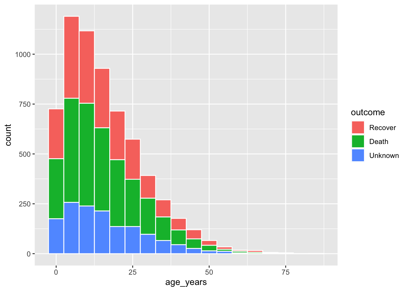
👀 Follow along 4.2 — The same with fill = "#2a78d6" in geom_histogram().
# Setting: every bar is blue
ggplot(data = linelist, mapping = aes(x = age_years)) +
  geom_histogram(binwidth = 5, fill = "#2a78d6", color = "white")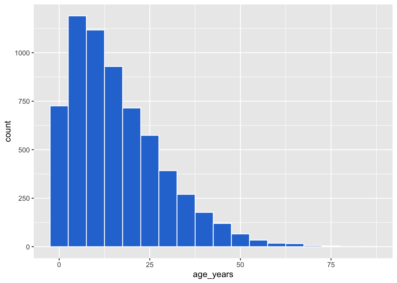
👀 Follow along 4.3 — What happens with fill = "blue" inside aes()? Open the box below and try it.
Note🤔 Think about it: what happens if you put
fill = "blue" inside aes()? Try it!
ggplot(data = linelist, mapping = aes(x = age_years, fill = "blue")) +
  geom_histogram(binwidth = 5)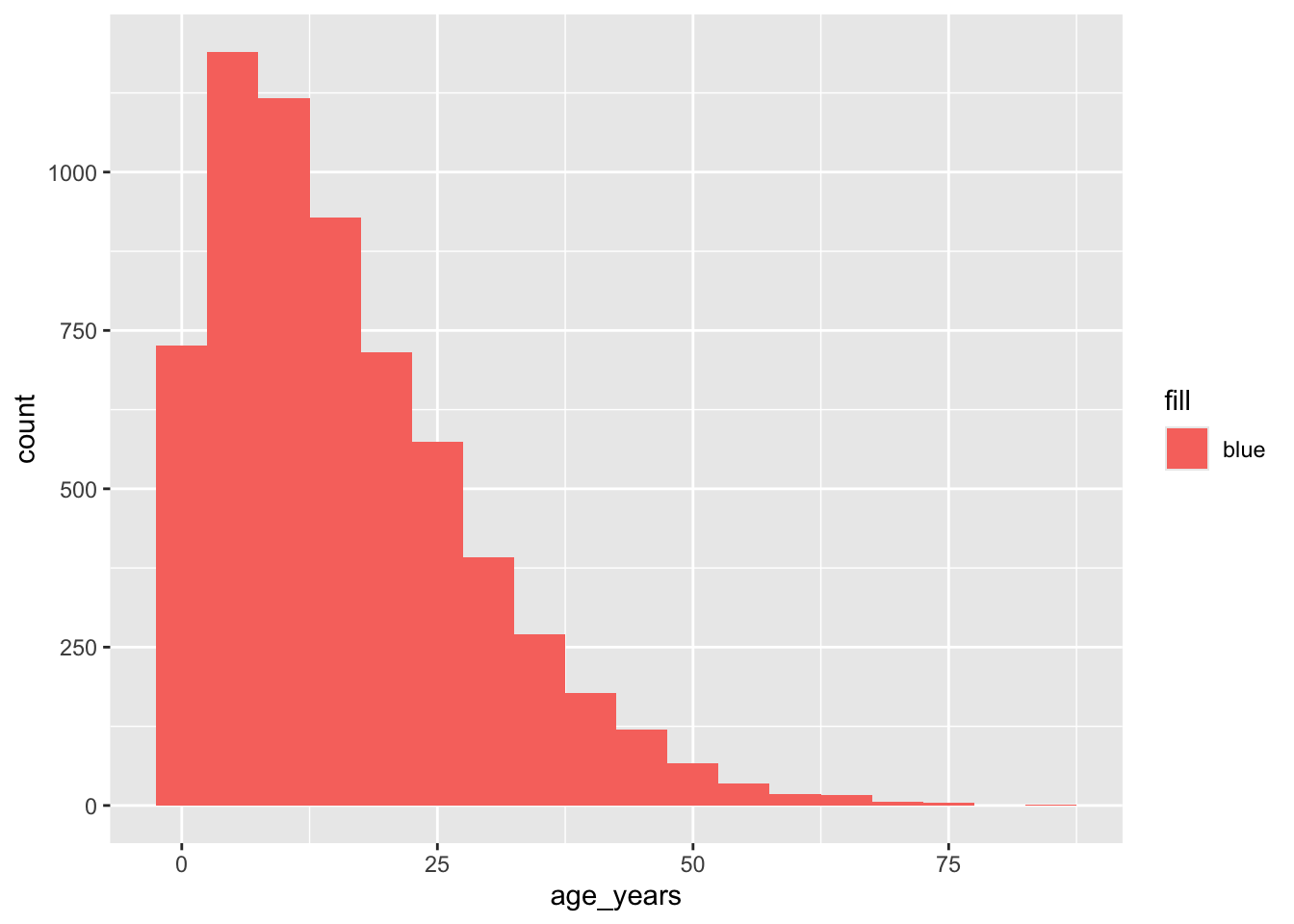
The bars are pink-red and the legend says “blue”! ggplot treated “blue” as data — a column whose every value is the word “blue” — and gave it the first default color.
WarningCommon mistakes
aes(fill = "blue")does not make blue bars. To use one fixed color, putfill = "blue"in thegeom_...(), outsideaes().
Important✏️ TRY IT 4 (3 min): mapping fill
Make a histogram of measles temp_c with binwidth = 0.2, then map fill = fever inside aes(). Why are there two “humps”?
✅ Check: the small hump near 37 °C is “no” fever; the big one near 39 °C is “yes”
NoteShow solution
ggplot(data = measles, mapping = aes(x = temp_c)) +
  geom_histogram(binwidth = 0.2, color = "white")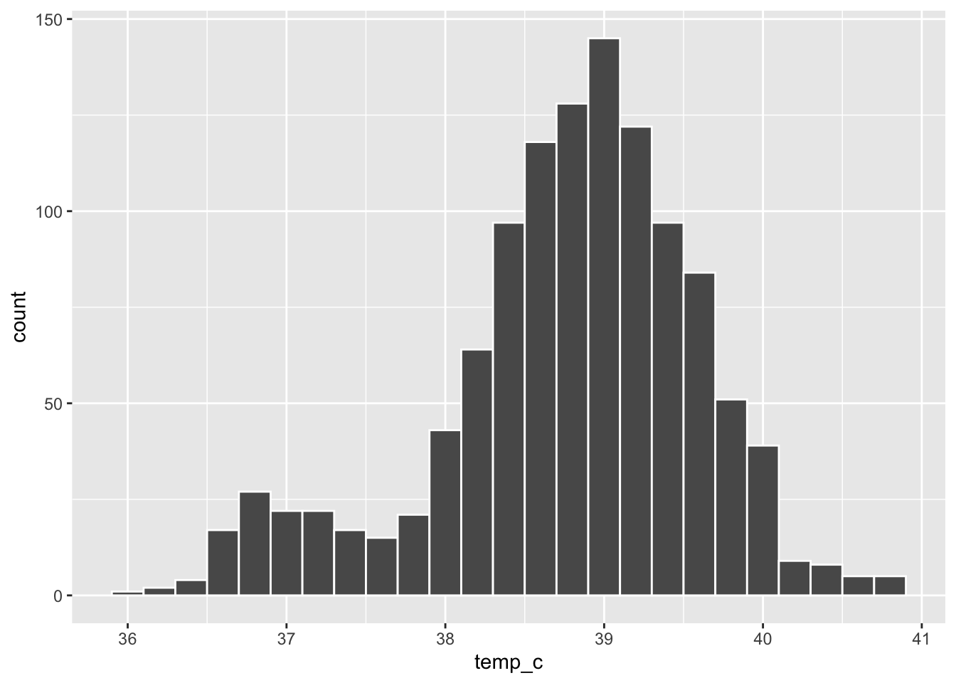
ggplot(data = measles, mapping = aes(x = temp_c, fill = fever)) +
  geom_histogram(binwidth = 0.2, color = "white")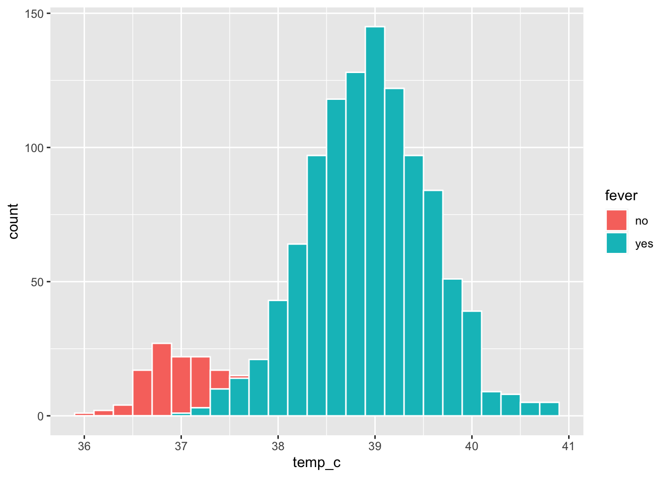
The small hump near 37 °C is the 99 patients without fever; the big hump near 39 °C is the 1064 patients with fever. Mapping fill to fever shows that the two humps are two groups.
Part 5: Scatter plots
A scatter plot shows the relationship between two numbers: one point per row.
👀 Follow along 5.1 — age_years vs wt_kg with geom_point().
ggplot(data = linelist, mapping = aes(x = age_years, y = wt_kg)) +
  geom_point()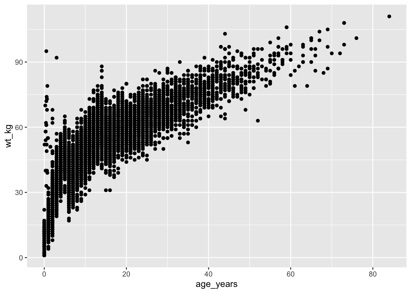
With 6,000+ points, many sit on top of each other. Make them smaller and see-through with size and alpha (0 = invisible, 1 = solid):
👀 Follow along 5.2 — Add size = 1 and alpha = 0.3; then map color = gender (the next two code blocks).
ggplot(data = linelist, mapping = aes(x = age_years, y = wt_kg)) +
  geom_point(size = 1, alpha = 0.3)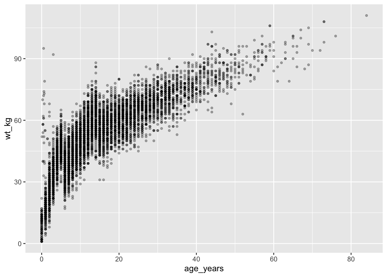
Map a third variable to color
ggplot(data = linelist, mapping = aes(x = age_years, y = wt_kg, color = gender)) +
  geom_point(size = 1, alpha = 0.4)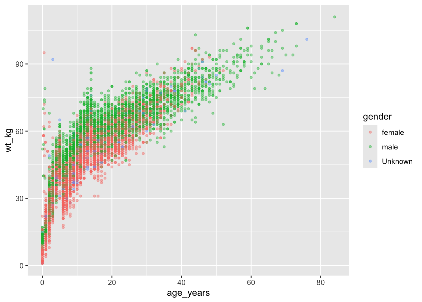
Add a trend line
geom_smooth() adds a trend line on top of the points. method = "lm" draws a straight line (linear model); se = FALSE hides the confidence band.
👀 Follow along 5.3 — Add geom_smooth(method = "lm", se = FALSE, color = "#eb6834").
ggplot(data = linelist, mapping = aes(x = age_years, y = wt_kg)) +
  geom_point(size = 1, alpha = 0.3) +
  geom_smooth(method = "lm", se = FALSE, color = "#eb6834")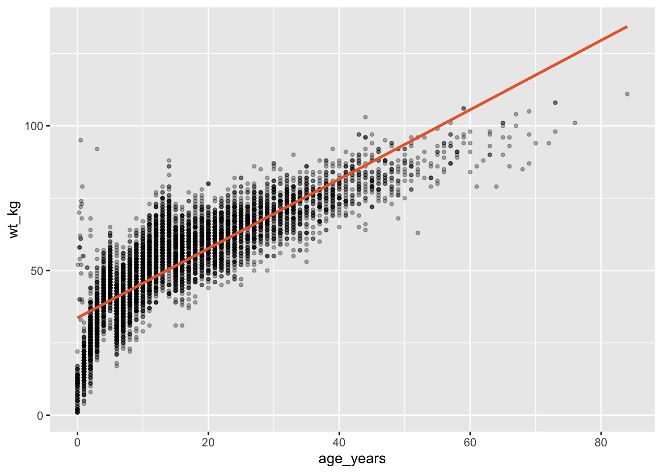
Filter right inside ggplot()
You can pipe data into ggplot(), so you can filter() first without making a new object:
👀 Follow along 5.4 — Only patients with fever: filter() first, then ggplot().
linelist %>%
  filter(fever == "yes") %>%
  ggplot(mapping = aes(x = age_years, y = wt_kg)) +
  geom_point(size = 1, alpha = 0.3)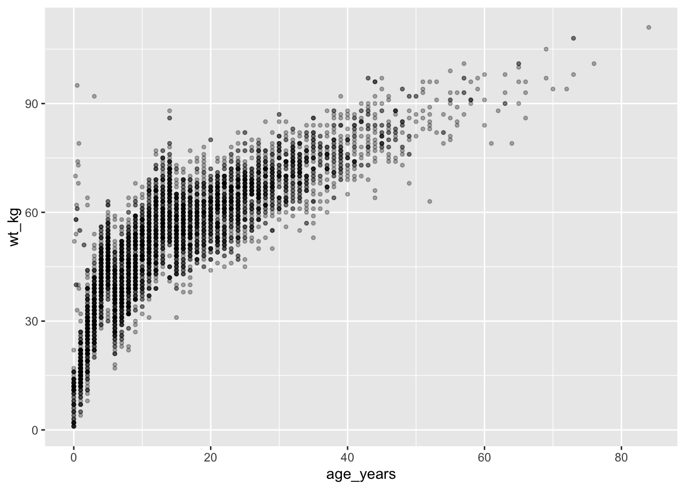
Notice the switch: %>% into ggplot(), then + between layers.
Important✏️ TRY IT 5 (4 min): a scatter plot
For hospitalized patients only (filter(!is.na(days_in_hospital))), plot age_years (x) against days_in_hospital (y) with alpha, and add a trend line. Is there a relationship?
✅ Check: 427 hospitalized patients; the trend line is almost flat (no relationship)
NoteShow solution
measles %>%
  filter(!is.na(days_in_hospital)) %>%
  ggplot(mapping = aes(x = age_years, y = days_in_hospital)) +
  geom_point(alpha = 0.3) +
  geom_smooth(method = "lm", se = FALSE, color = "#eb6834")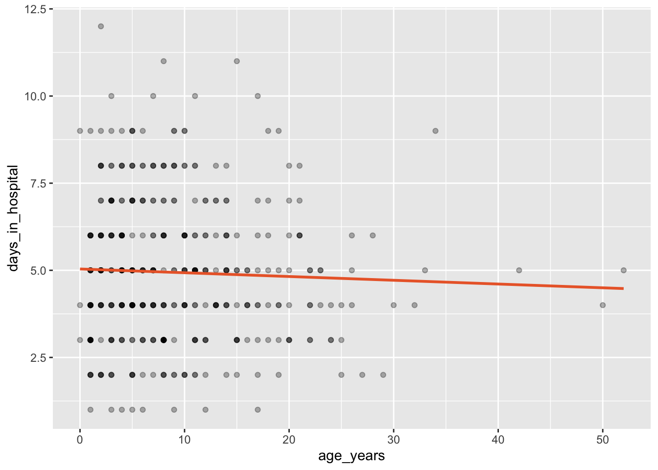
The trend line is almost flat: older and younger patients stay in hospital about as long. “No relationship” is a result too!
Part 6: Box plots
A box plot compares the distribution of a number across groups:
- The thick line is the median
- The box holds the middle 50% of values (from the 25th to the 75th percentile — the IQR)
- The whiskers reach the most extreme values within 1.5 × IQR of the box
- Points beyond the whiskers are possible outliers
👀 Follow along 6.1 — age_years by gender with geom_boxplot().
ggplot(data = linelist, mapping = aes(x = gender, y = age_years)) +
  geom_boxplot()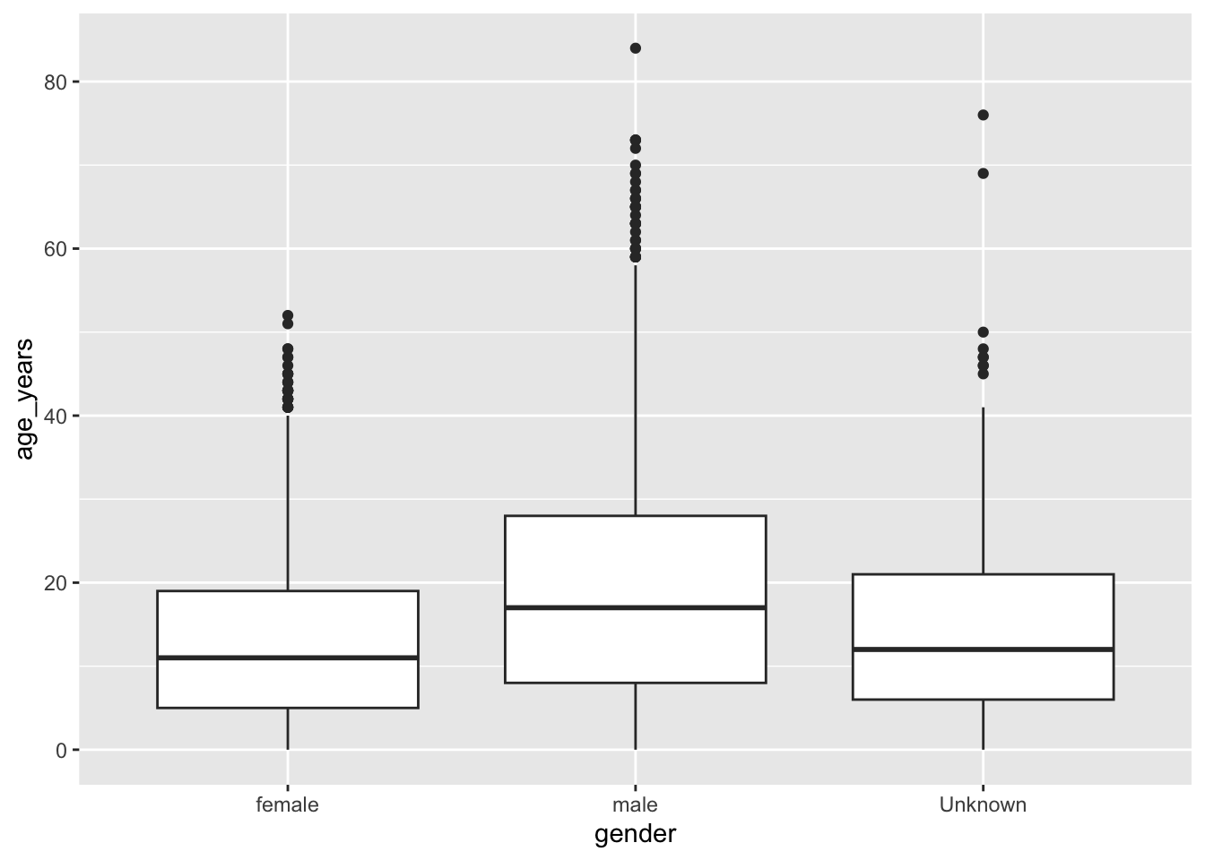
Clean it up
Remove the “Unknown” group, color the boxes, and drop the legend (the x-axis already names the groups):
👀 Follow along 6.2 — Filter out “Unknown”, add fill = gender, and remove the legend.
linelist %>%
  filter(gender != "Unknown") %>%
  ggplot(mapping = aes(x = gender, y = age_years, fill = gender)) +
  geom_boxplot() +
  theme(legend.position = "none")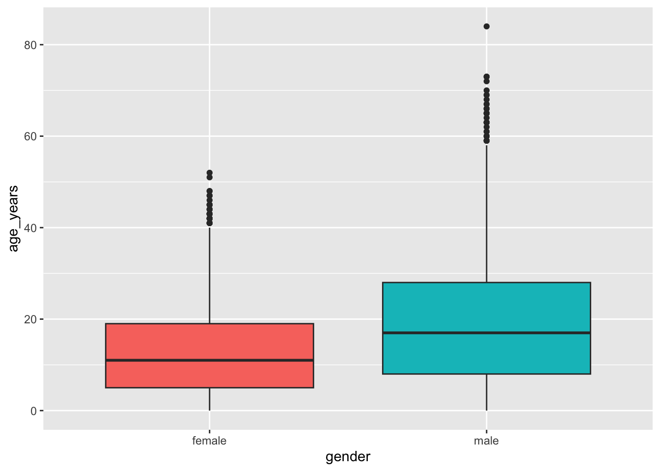
Add the mean
stat_summary() calculates a statistic for each group and draws it. Here, the mean as a diamond:
👀 Follow along 6.3 — Add the mean with stat_summary().
linelist %>%
  filter(gender != "Unknown") %>%
  ggplot(mapping = aes(x = gender, y = age_years, fill = gender)) +
  geom_boxplot() +
  stat_summary(fun = mean, geom = "point", shape = 23, size = 3, fill = "white") +
  theme(legend.position = "none")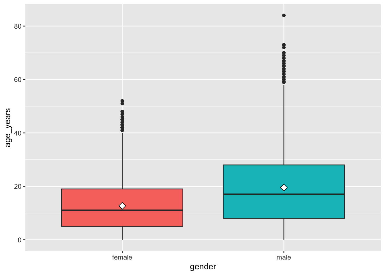
Note
geom_violin() shows the full shape of each distribution. Try swapping it in for geom_boxplot().
Important✏️ TRY IT 6 (4 min): a box plot
Make a box plot of days_in_hospital by vaccinated (hospitalized patients only), with the mean and no legend.
✅ Check: three boxes; the medians are 4–5 days for every group
NoteShow solution
measles %>%
  filter(!is.na(days_in_hospital)) %>%
  ggplot(mapping = aes(x = vaccinated, y = days_in_hospital, fill = vaccinated)) +
  geom_boxplot() +
  stat_summary(fun = mean, geom = "point", shape = 23, size = 3, fill = "white") +
  theme(legend.position = "none")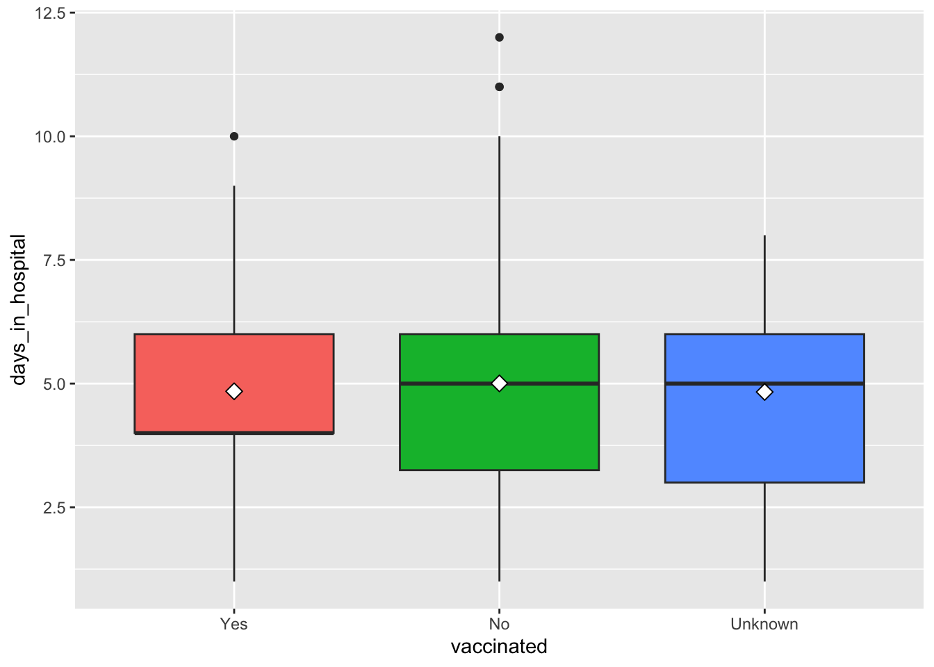
The medians are 4 days (Yes) and 5 days (No, Unknown), and the means are all about 5: no clear difference in hospital stay by vaccination status. The boxes appear in the order you set with fct_relevel() in Part 1.
Part 7: Labels and themes
labs()
👀 Follow along 7.1 — Add labs() to the box plot.
linelist %>%
  filter(gender != "Unknown") %>%
  ggplot(mapping = aes(x = gender, y = age_years, fill = gender)) +
  geom_boxplot() +
  labs(
    title    = "Age distribution by gender",
    subtitle = "Cases with known gender",
    x        = "Gender",
    y        = "Age (years)",
    caption  = "Source: workshop outbreak linelist"
  ) +
  theme(legend.position = "none")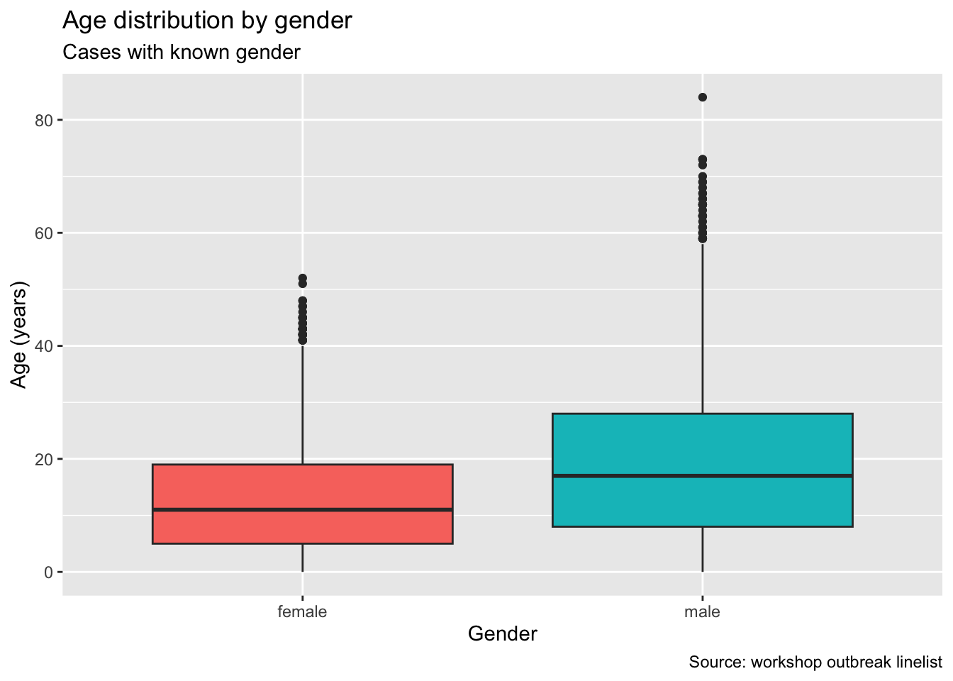
Themes
A theme changes the look of everything that isn’t data: background, grid lines, fonts. Try theme_minimal(), theme_classic(), theme_bw(), and theme_light().
👀 Follow along 7.2 — Try theme_minimal(), theme_classic(), and theme_bw() on the age histogram.
ggplot(data = linelist, mapping = aes(x = age_years)) +
  geom_histogram(binwidth = 5, fill = "#2a78d6", color = "white") +
  labs(
    title = "Age distribution of cases",
    x     = "Age (years)",
    y     = "Number of cases"
  ) +
  theme_minimal(base_size = 14)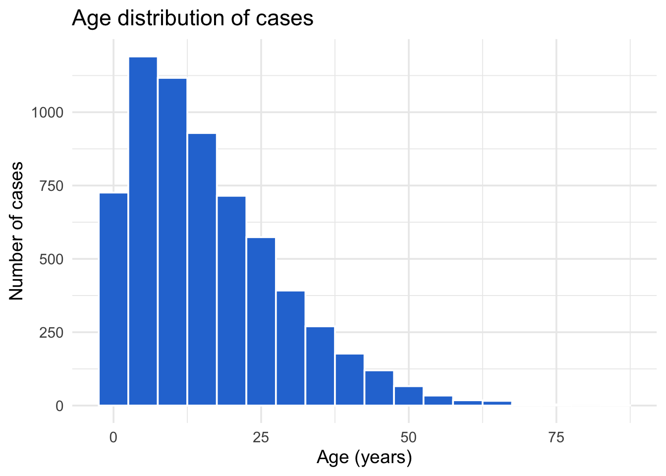
base_size makes all the text bigger — useful for slides.
WarningOrder matters
A complete theme like theme_minimal() resets everything, so put it before theme(legend.position = ...) or your change will be overwritten.
Save a plot as an object
A plot can be saved with <- and built on later:
👀 Follow along 7.3 — Save a plot as age_plot, then add labs() and a theme to it.
age_plot <- ggplot(data = linelist, mapping = aes(x = age_years)) +
  geom_histogram(binwidth = 5, fill = "#2a78d6", color = "white")

age_plot +
  labs(title = "Age distribution of cases", x = "Age (years)", y = "Number of cases") +
  theme_minimal()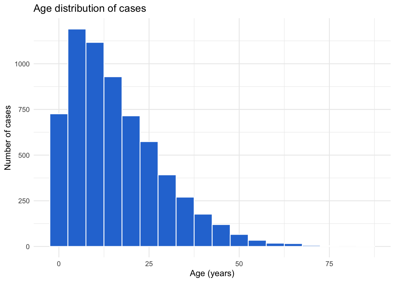
Important✏️ TRY IT 7 (5 min): finish a plot
Finish one of your measles plots with a title, subtitle, axis labels, a caption, and a theme. Save it as my_plot.
✅ Check: typing my_plot in the Console shows your finished plot
NoteShow solution
my_plot <- ggplot(data = measles, mapping = aes(x = temp_c, fill = fever)) +
  geom_histogram(binwidth = 0.2, color = "white") +
  labs(
    title    = "Temperature of measles cases",
    subtitle = "Patients with fever cluster around 39 °C",
    x        = "Temperature (°C)",
    y        = "Number of cases",
    fill     = "Fever",
    caption  = "Source: practice measles linelist"
  ) +
  theme_minimal()

my_plot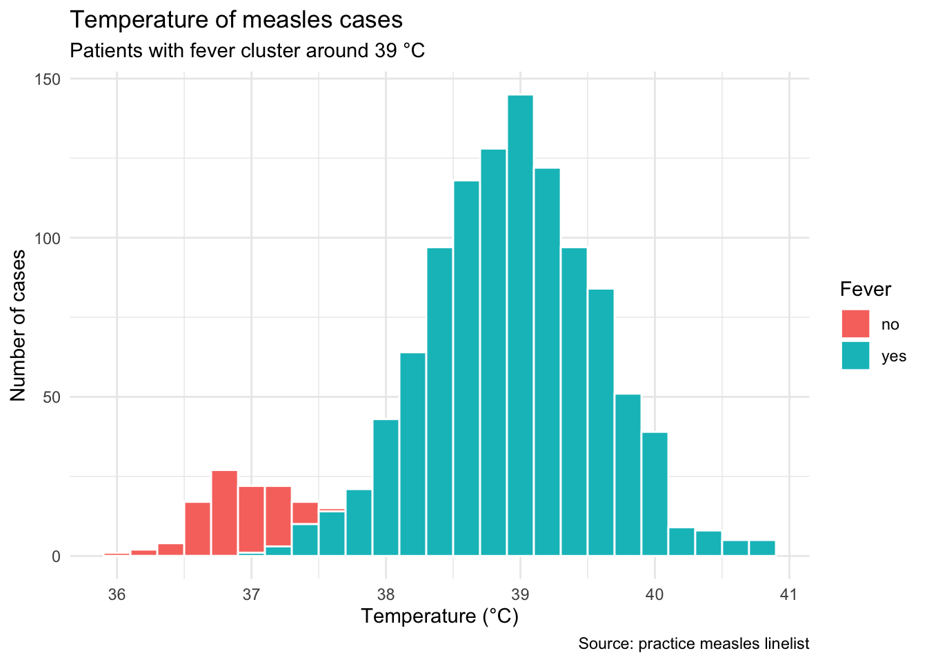
This is one example — any measles plot works. fill = "Fever" inside labs() renames the legend title. Saving the plot as my_plot stores it in the Variables pane, and typing its name draws it.
Tip⭐ Bonus
- Make the measles age histogram with
fill = vaccinated. Which ages have the most unvaccinated cases? - Swap
geom_boxplot()forgeom_violin()in your box plot. What does it show? - Brought your own data? Make a histogram, a scatter plot, and a box plot.
See the solutions file for the code.
Key points
- Every ggplot needs data, aesthetics (
aes()), and a geometry (geom_...()); layers are joined with+, not%>%. geom_histogram()shows the distribution of one number — choose thebinwidthyourself.- Mapping (inside
aes()) lets a column control color and adds a legend; setting (outsideaes()) uses one fixed color. geom_point()shows the relationship between two numbers;alphaandsizehelp with overlapping points, andgeom_smooth(method = "lm")adds a trend line.geom_boxplot()compares a number across groups;stat_summary()adds the mean.labs()adds titles and axis labels, and a complete theme liketheme_minimal()changes the overall look (put it beforetheme(...)changes).- You can pipe data into
ggplot()tofilter()first, and save a plot as an object with<-.
Next: Session 7 — Plotting further. We make bar charts, choose colors, draw epidemic curves, split plots into facets, and save plots to files.