library(tidyverse)
library(here)
library(rio)

linelist <- import(here("processed_data", "combined_linelist.rds"), trust = TRUE) %>%
  mutate(
    age_cat = fct_relevel(age_cat, "Under 18", "18-29", "30-39", "40-49",
                          "50-59", "60-69", "70-79", "80+", "Unknown"),
    outcome = fct_relevel(outcome, "Recover", "Death", "Unknown")
)Session 7: Plotting Further — Bar Charts, Colors, Epicurves, and Facets
Bar charts of counts and values, choosing colors, epidemic curves, facets, and saving plots
NoteIn this session you will learn to
- Make bar charts of counts (
geom_bar()) and of values you calculated (geom_col()) - Order bars sensibly and choose stacked, side-by-side, or 100% bars
- Choose colors on purpose with
scale_fill_manual() - Make an epidemic curve from dates
- Split a plot into small multiples with
facet_wrap() - Save plots to files with
ggsave()
Before you start: open the workshop folder in Positron (File → Open Folder…) and open student_scripts/Session 7 - Plotting Further_STUDENT.R. This session starts from processed_data/combined_linelist.rds and processed_data/measles_final.rds, the files you made in Session 3. Missed a session? Ready-made copies are already in processed_data/.
Where this session fits. Most data projects go through the same steps, whatever the topic. Today covers Visualize and Save and share (highlighted): more kinds of plots, chosen colors, and saving plots to files you can put in a report.
- Import
- Inspect
- Clean
- Combine
- Reshape
- Summarize
- Visualize
- Save and share
- Automate
Part 1: Set up
Load the packages, import the finished linelist, and put the categories in a sensible order (the same as Session 6):
👀 Follow along 1.1 — Load tidyverse, here, and rio; import combined_linelist.rds as linelist, and fct_relevel() age_cat and outcome (same as Session 6).
TipSave your colors once
Saving your colors in a named vector means every plot uses the same color for the same category:
vacc_colors <- c("Yes" = "#2a78d6", "No" = "#eb6834", "Unknown" = "#9a9a95")
You will use these colors in Part 4.
Part 2: Bar charts of counts: geom_bar()
geom_bar() counts the rows in each category for you — you only give it x.
👀 Follow along 2.1 — geom_bar() with x = hospital_name, then with y = hospital_name (the next two code blocks).
ggplot(data = linelist, mapping = aes(x = hospital_name)) +
  geom_bar()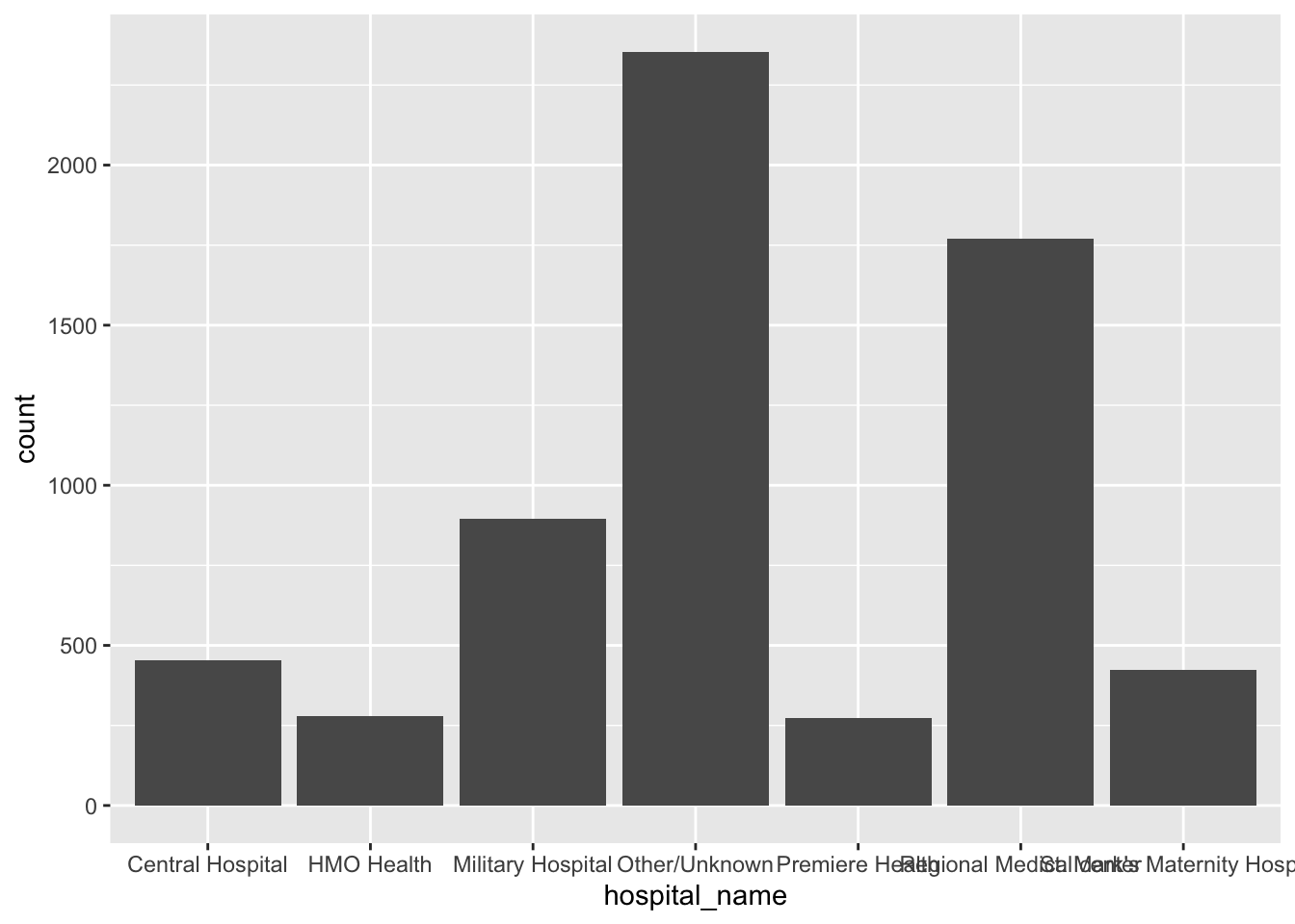
The labels overlap. Put the categories on the y-axis instead to get horizontal bars:
ggplot(data = linelist, mapping = aes(y = hospital_name)) +
  geom_bar()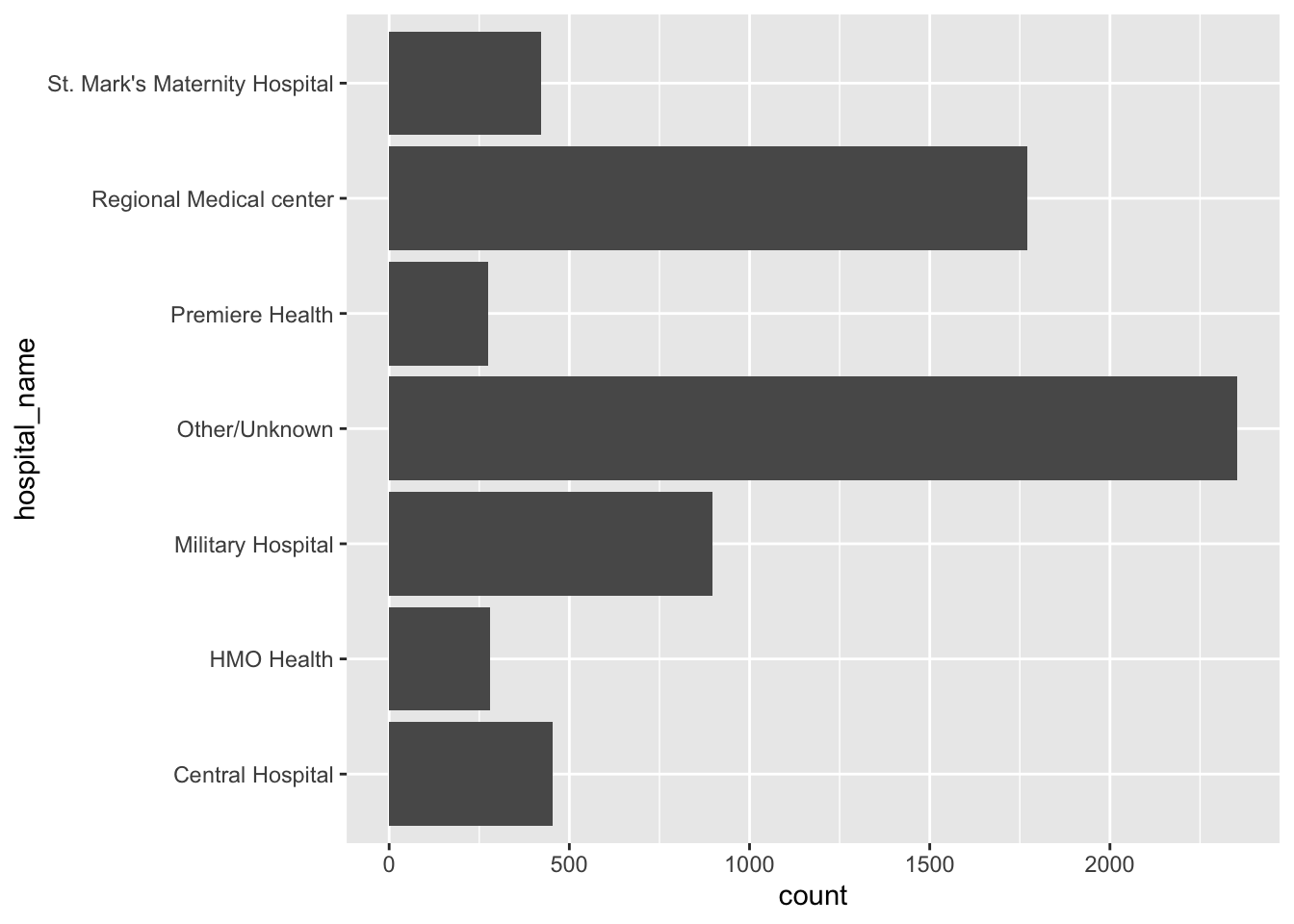
Order the bars
Alphabetical order rarely helps. fct_infreq() orders by count (most common first), and fct_rev() flips it so the longest bar is at the top:
👀 Follow along 2.2 — Order the bars with fct_rev(fct_infreq(hospital_name)), and add a fill color and labs().
ggplot(data = linelist, mapping = aes(y = fct_rev(fct_infreq(hospital_name)))) +
  geom_bar(fill = "#2a78d6") +
  labs(title = "Cases by hospital", x = "Number of cases", y = NULL) +
  theme_minimal()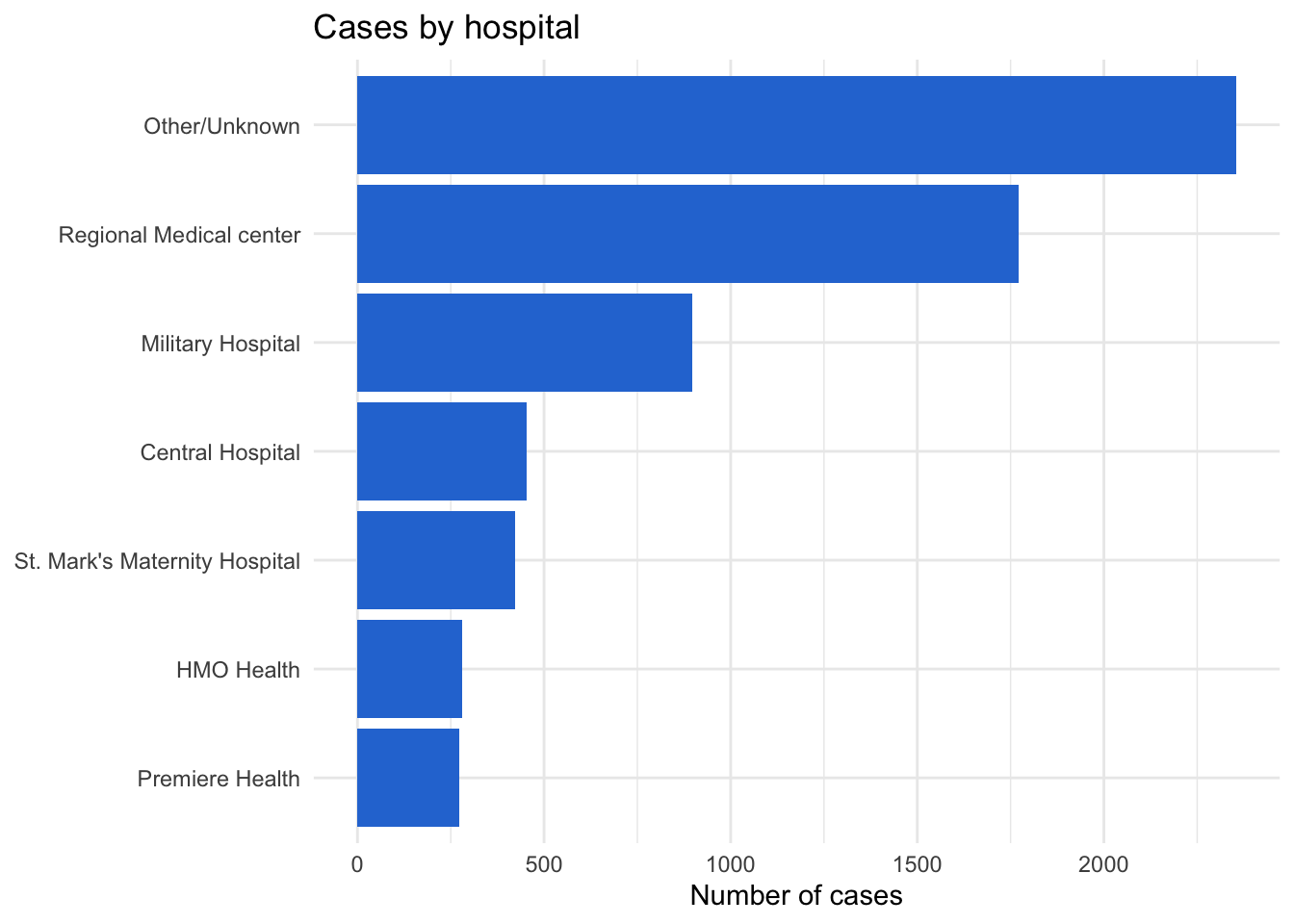
Fill by a second variable
Map fill to split each bar. The position argument controls how the pieces are arranged:
👀 Follow along 2.3 — x = age_cat, fill = outcome, with position = "stack", "fill", and "dodge" (the next three code blocks).
# "stack" (the default): counts, stacked
ggplot(data = linelist, mapping = aes(x = age_cat, fill = outcome)) +
  geom_bar(position = "stack")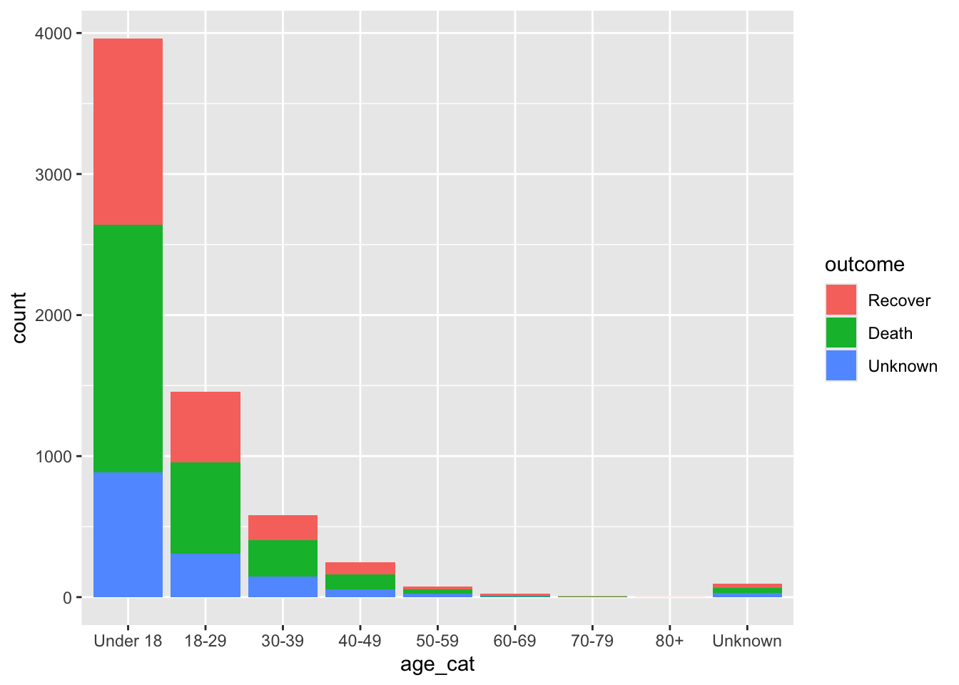
# "fill": every bar is 100% — compares PROPORTIONS across groups
ggplot(data = linelist, mapping = aes(x = age_cat, fill = outcome)) +
  geom_bar(position = "fill")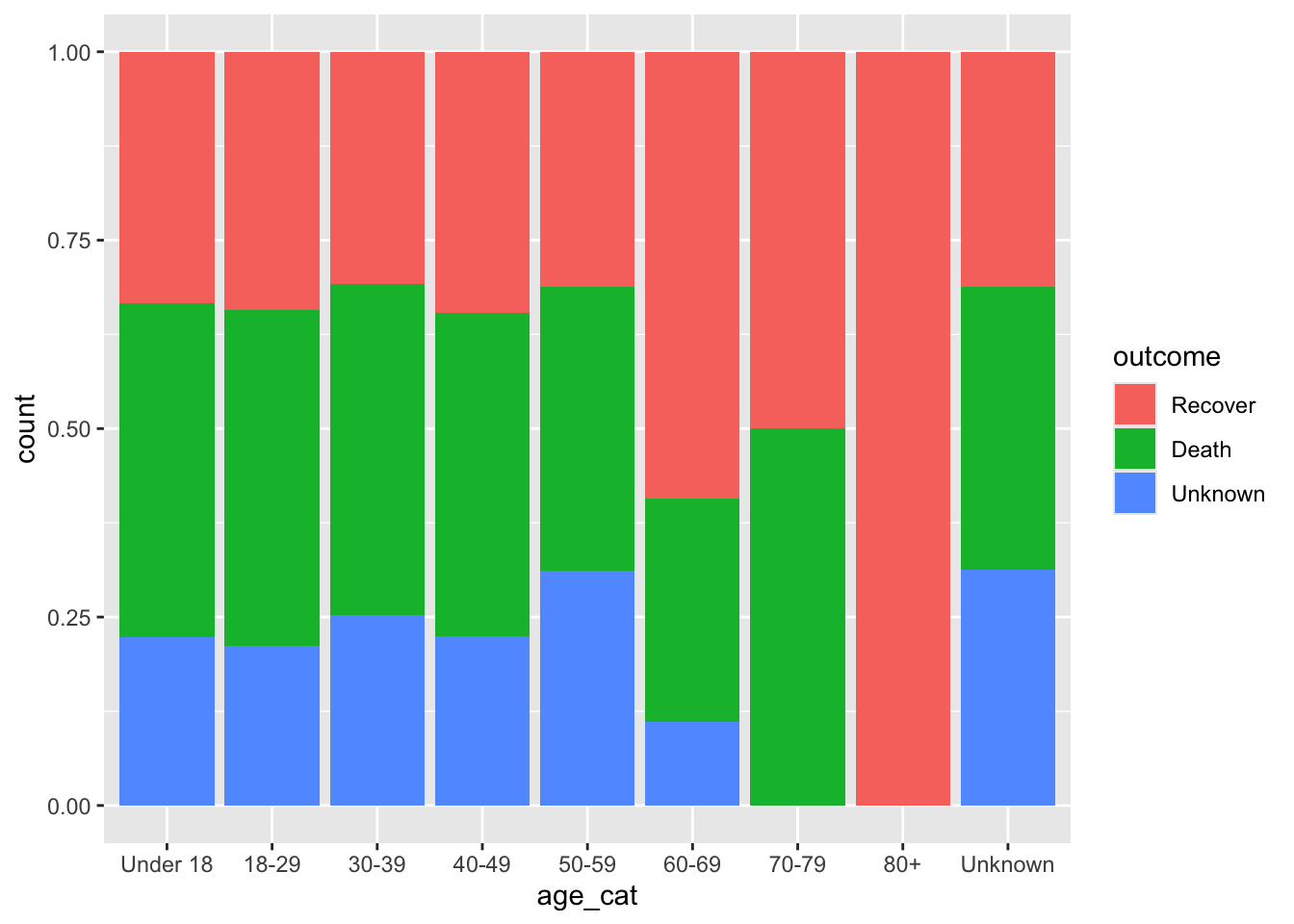
# "dodge": side by side — compares COUNTS within each group
ggplot(data = linelist, mapping = aes(x = age_cat, fill = outcome)) +
  geom_bar(position = "dodge")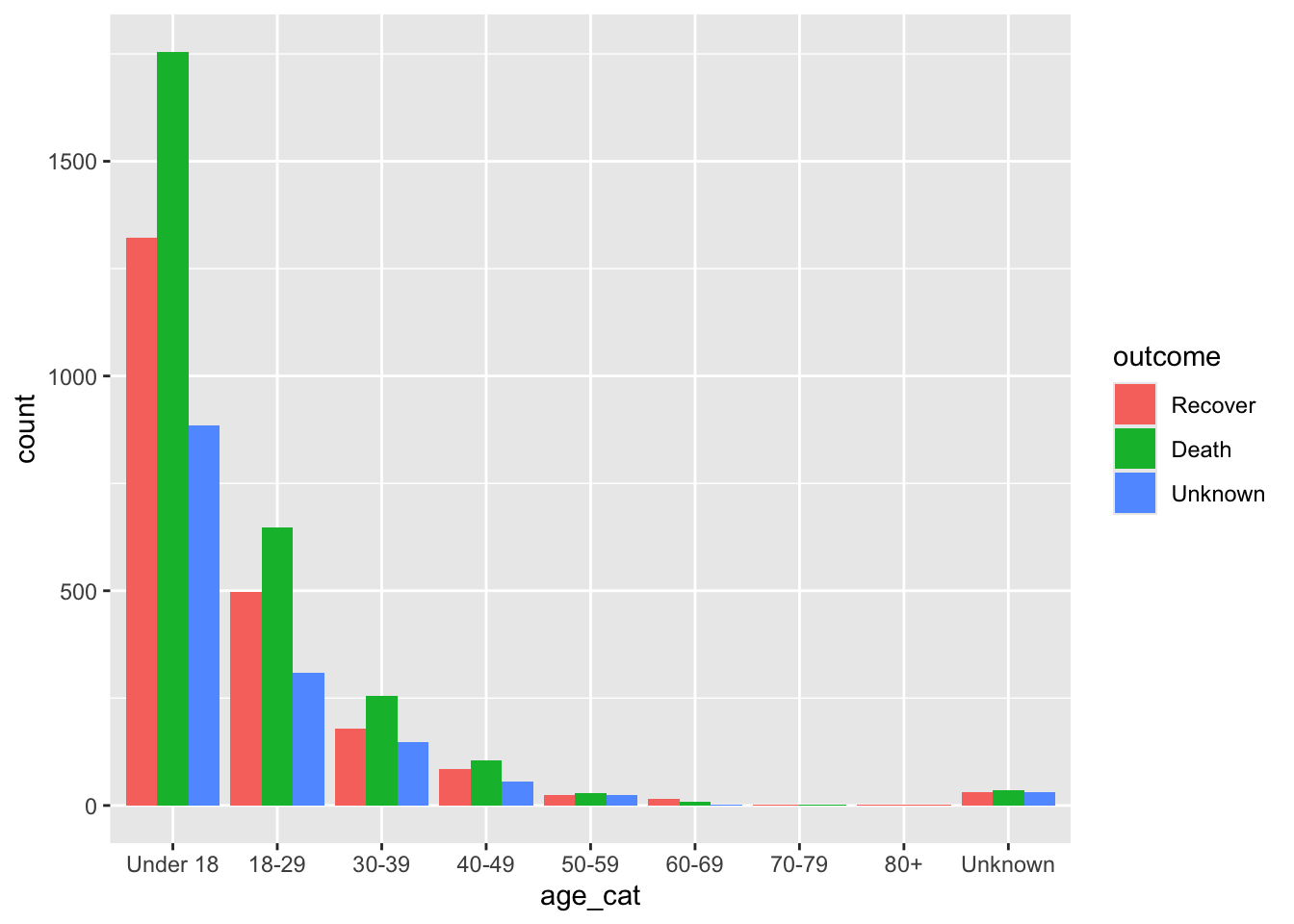
Important✏️ TRY IT 2 (3 min): cases by district
Make a horizontal bar chart of measles cases by district, longest bar on top.
✅ Check: North is at the top; Unknown is at the bottom
NoteShow solution
ggplot(data = measles, mapping = aes(y = fct_rev(fct_infreq(district)))) +
  geom_bar(fill = "#2a78d6") +
  labs(title = "Measles cases by district", x = "Number of cases", y = NULL) +
  theme_minimal()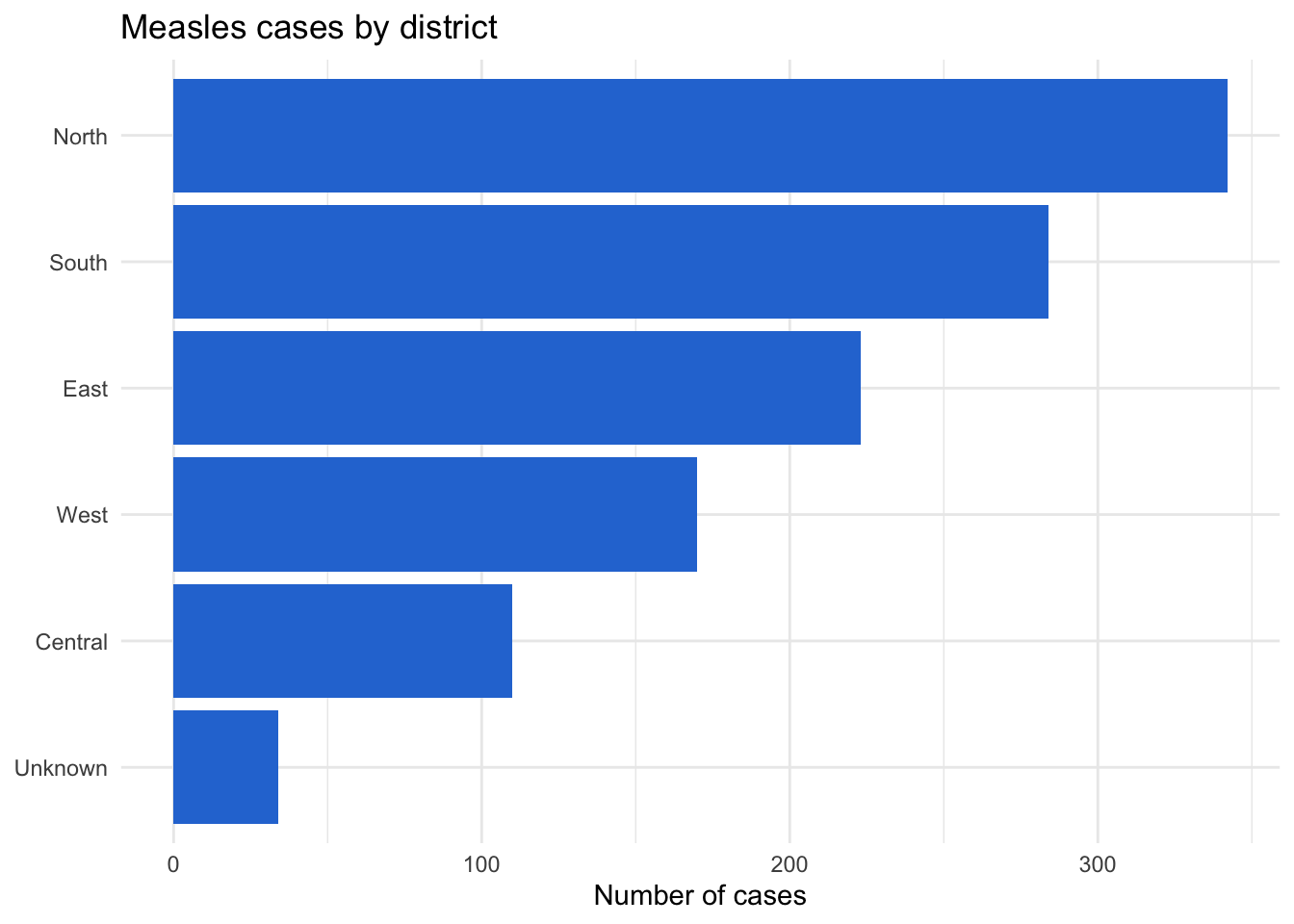
fct_infreq() puts North (342 cases) first, and fct_rev() moves it to the top. Unknown (34 cases) ends up at the bottom.
Part 3: Bar charts of values: geom_col()
When you have already calculated the numbers (with count() or summarise() from Session 5), use geom_col() and give it both x and y:
👀 Follow along 3.1 — Create death_by_age (the percentage who died in each age group), then plot it with geom_col().
death_by_age <- linelist %>%
  filter(outcome != "Unknown", age_cat != "Unknown") %>%
  group_by(age_cat) %>%
  summarise(
    n         = n(),
    pct_death = mean(outcome == "Death") * 100
  )

death_by_age
# A tibble: 8 × 3
age_cat n pct_death
<fct> <int> <dbl>
1 Under 18 3077 57.0
2 18-29 1146 56.5
3 30-39 435 58.9
4 40-49 190 55.3
5 50-59 53 54.7
6 60-69 24 33.3
7 70-79 6 50
8 80+ 1 0 ggplot(data = death_by_age, mapping = aes(x = age_cat, y = pct_death)) +
geom_col(fill = "#2a78d6") +
labs(title = "Case fatality by age group", x = "Age group", y = "Deaths (% of cases)") +
theme_minimal()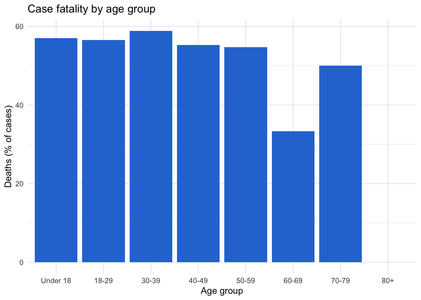
Note
geom_bar() or geom_col()?
geom_bar() counts rows for you (one row per patient): give it x only. geom_col() draws numbers you already have (one row per bar): give it x and y.
fct_reorder(CATEGORY, NUMBER) sorts the bars by the number.
Important✏️ TRY IT 3 (5 min): case rates by district
- Calculate cases per 10,000 people by district (Session 5), leaving out “Unknown”.
- Plot it with
geom_col(), usingx = fct_reorder(district, rate_per_10k).
✅ Check: bars from Central (lowest, 5.2) to East (highest, 22.8)
NoteShow solution
# a)
district_rates <- measles %>%
  filter(district != "Unknown") %>%
  count(district, population) %>%
  mutate(rate_per_10k = round(n / population * 10000, 1))

district_rates
district population n rate_per_10k
1 Central 210000 110 5.2
2 East 98000 223 22.8
3 North 185000 342 18.5
4 South 142000 284 20.0
5 West 76500 170 22.2# b)
ggplot(data = district_rates, mapping = aes(x = fct_reorder(district, rate_per_10k), y = rate_per_10k)) +
geom_col(fill = "#2a78d6") +
labs(
title = "Measles cases per 10,000 people by district",
x = "District",
y = "Cases per 10,000 people"
) +
theme_minimal()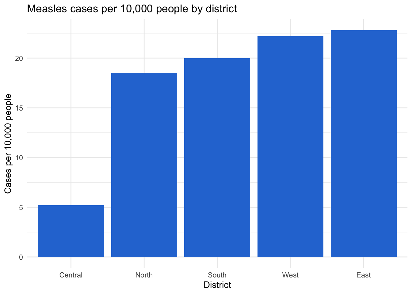
count() makes one row per district, so geom_col() is the right choice. North has the most cases, but Central has the largest population, so the rates tell a different story: East (22.8) and West (22.2) are highest, Central (5.2) is lowest.
Part 4: Choosing colors
ggplot’s default colors are fine for exploring, but for a report choose colors on purpose:
- Use colors that people with color-vision deficiency can tell apart. Avoid red vs green (the most common problem pair) and two shades of the same color. Blue (
#2a78d6) and orange (#eb6834) are a safe pair - Give “Unknown” or “Other” a gray (
#9a9a95), so it doesn’t compete with the real categories - Keep the same color for the same category in every plot of a report
scale_fill_manual() (for fill) and scale_color_manual() (for color) set the colors by name:
👀 Follow along 4.1 — Save outcome_colors, then make a 100% bar chart of outcome by age_cat with scale_fill_manual(), a white outline, and a percent y-axis.
outcome_colors <- c("Recover" = "#2a78d6", "Death" = "#eb6834", "Unknown" = "#9a9a95")

ggplot(data = linelist, mapping = aes(x = age_cat, fill = outcome)) +
  geom_bar(position = "fill", color = "white") +
  scale_fill_manual(values = outcome_colors) +
  scale_y_continuous(labels = scales::percent) +
  labs(
    title = "Outcome by age group",
    x     = "Age group",
    y     = "Percent of cases",
    fill  = "Outcome"
  ) +
  theme_minimal()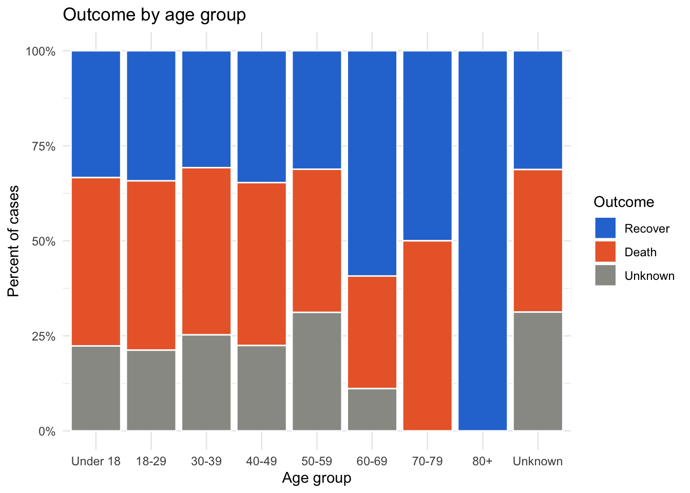
TipNeed more colors?
The viridis scales are built into ggplot2 and are colorblind-friendly: try scale_fill_viridis_d() for categories.
Rotate long labels
If you keep labels on the x-axis, rotate them so they don’t overlap:
ggplot(data = linelist, mapping = aes(x = hospital_name)) +
  geom_bar(fill = "#2a78d6") +
  theme_minimal() +
  theme(axis.text.x = element_text(angle = 45, hjust = 1))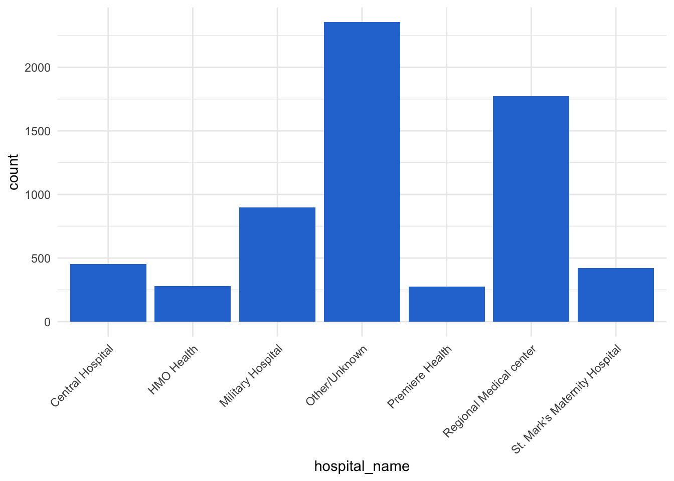
Important✏️ TRY IT 4 (4 min): vaccination by age group
Make a 100% bar chart of vaccinated by age_cat, with vacc_colors, a percent y-axis, labels, and theme_minimal().
✅ Check: every bar reaches 100%; “Yes” is blue in every bar
NoteShow solution
ggplot(data = measles, mapping = aes(x = age_cat, fill = vaccinated)) +
  geom_bar(position = "fill", color = "white") +
  scale_fill_manual(values = vacc_colors) +
  scale_y_continuous(labels = scales::percent) +
  labs(
    title = "Vaccination status of measles cases by age group",
    x     = "Age group",
    y     = "Percent of cases",
    fill  = "Vaccinated"
  ) +
  theme_minimal()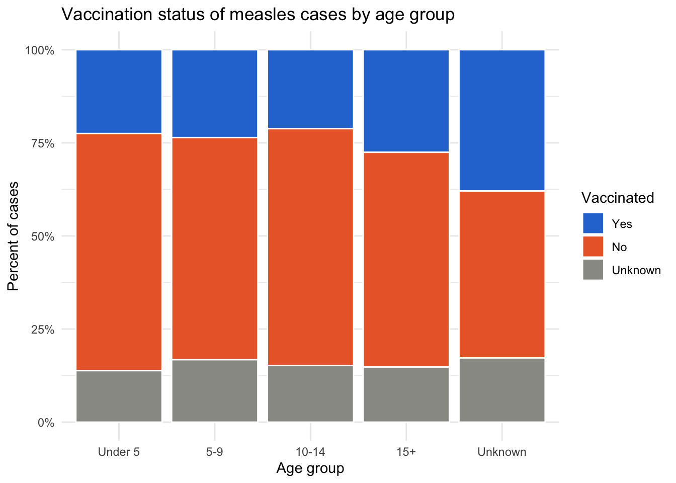
position = "fill" makes every bar 100%, and because vacc_colors is a named vector, “Yes” is always blue, “No” orange, and “Unknown” gray.
Part 5: Epidemic curves
An epidemic curve (epicurve) shows the number of new cases over time — the most important plot in outbreak investigation. It is a histogram of a date column:
👀 Follow along 5.1 — geom_histogram() of onset_date with binwidth = 7. What’s going on before 2014?
ggplot(data = linelist, mapping = aes(x = onset_date)) +
  geom_histogram(binwidth = 7, fill = "#2a78d6", color = "white")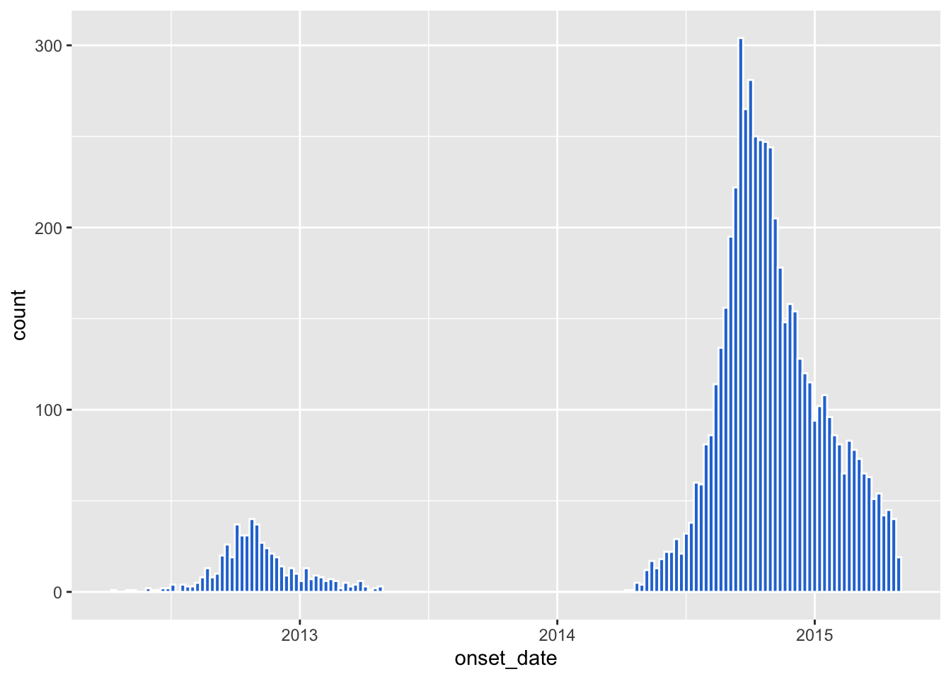
Zoom in on the outbreak and format the date axis:
👀 Follow along 5.2 — Keep onset dates from 2014, and add scale_x_date() and labs().
linelist %>%
  filter(onset_date >= as.Date("2014-01-01")) %>%
  ggplot(mapping = aes(x = onset_date)) +
  geom_histogram(binwidth = 7, fill = "#2a78d6", color = "white") +
  scale_x_date(date_breaks = "2 months", date_labels = "%b\n%Y") +
  labs(
    title    = "Epidemic curve: weekly cases by date of symptom onset",
    subtitle = "Onset dates from 2014 onward",
    x        = "Week of onset",
    y        = "Number of cases"
  ) +
  theme_minimal()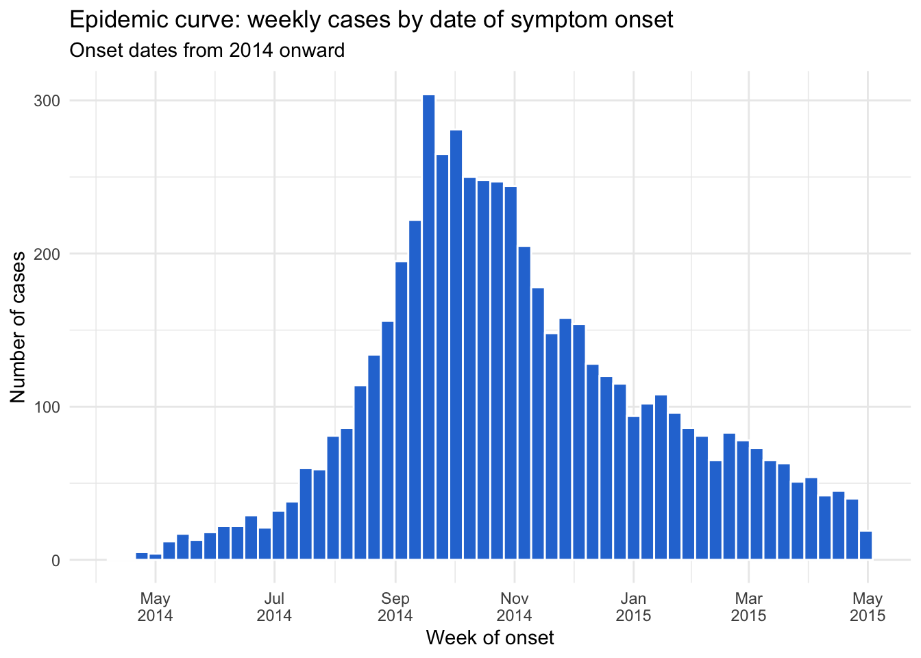
Epicurve by outcome
👀 Follow along 5.3 — Fill the epicurve by outcome with outcome_colors.
linelist %>%
  filter(onset_date >= as.Date("2014-01-01")) %>%
  ggplot(mapping = aes(x = onset_date, fill = outcome)) +
  geom_histogram(binwidth = 7, color = "white") +
  scale_fill_manual(values = outcome_colors) +
  scale_x_date(date_breaks = "2 months", date_labels = "%b\n%Y") +
  labs(x = "Week of onset", y = "Number of cases", fill = "Outcome") +
  theme_minimal()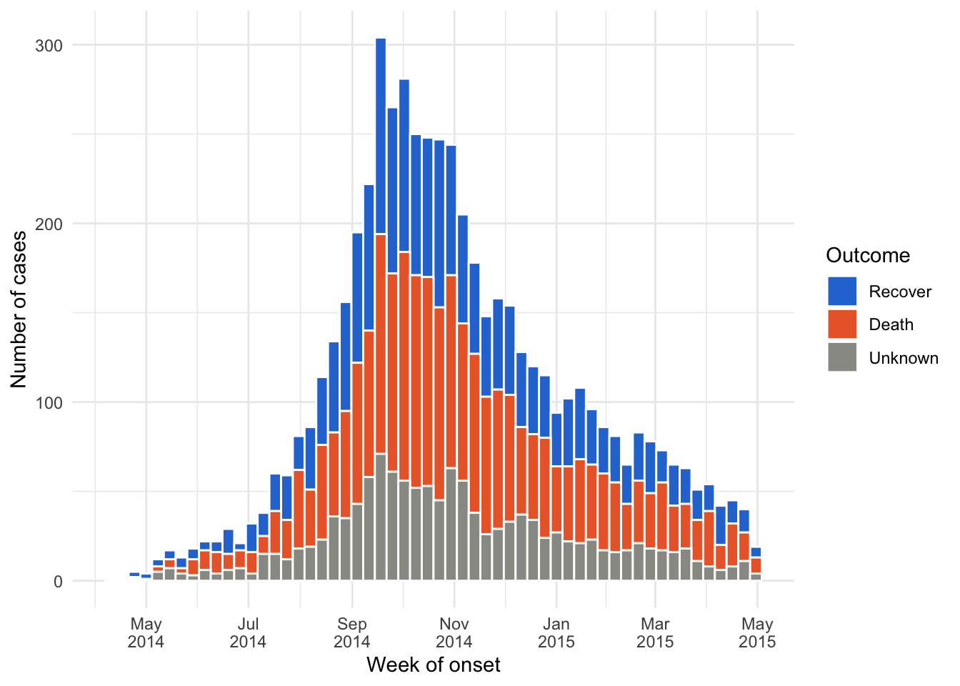
Important✏️ TRY IT 5 (5 min): the measles epicurve
Make a weekly epicurve of measles report_date, filled by vaccinated, with vacc_colors and scale_x_date(date_breaks = "1 month", date_labels = "%b"). Save it as measles_epicurve — you will need it in Part 7. Hint: filter(!is.na(report_date)) first. When did the outbreak peak?
✅ Check: the peak is in the second half of March (about 115 cases in one week)
NoteShow solution
measles_epicurve <- measles %>%
  filter(!is.na(report_date)) %>%
  ggplot(mapping = aes(x = report_date, fill = vaccinated)) +
  geom_histogram(binwidth = 7, color = "white") +
  scale_fill_manual(values = vacc_colors) +
  scale_x_date(date_breaks = "1 month", date_labels = "%b") +
  labs(
    title = "Measles cases by week of report, 2024",
    x     = "Week of report",
    y     = "Number of cases",
    fill  = "Vaccinated"
  ) +
  theme_minimal()

measles_epicurve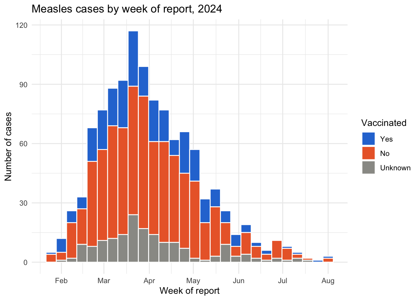
The outbreak peaked in the second half of March 2024, with 117 cases in the peak week. Saving the plot as an object means it only appears when you print it (the last line).
Part 6: Facets
facet_wrap() splits one plot into small multiples — one panel per category, all with the same axes so they are easy to compare:
👀 Follow along 6.1 — The epicurve with facet_wrap(~ hospital_name), leaving out “Other/Unknown”.
linelist %>%
  filter(onset_date >= as.Date("2014-01-01"), hospital_name != "Other/Unknown") %>%
  ggplot(mapping = aes(x = onset_date)) +
  geom_histogram(binwidth = 7, fill = "#2a78d6", color = "white") +
  facet_wrap(~ hospital_name) +
  scale_x_date(date_breaks = "4 months", date_labels = "%b\n%Y") +
  labs(title = "Weekly cases by hospital", x = "Week of onset", y = "Number of cases") +
  theme_minimal()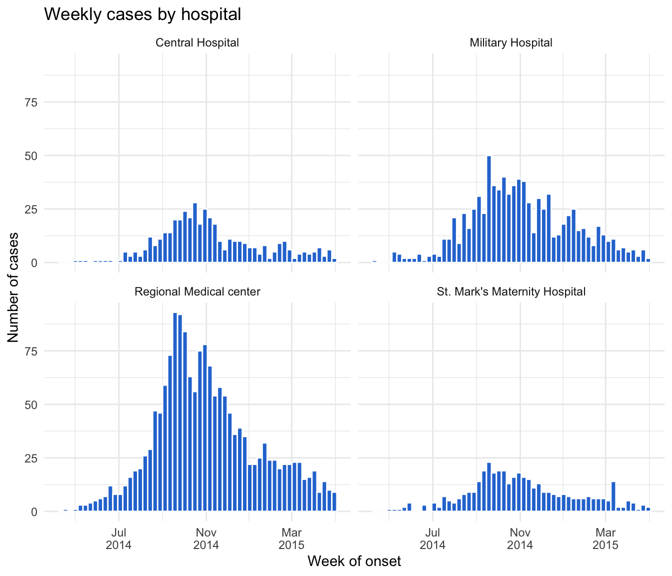
Facets work with any plot:
👀 Follow along 6.2 — An age histogram with facet_wrap(~ gender), leaving out “Unknown”.
linelist %>%
  filter(gender != "Unknown") %>%
  ggplot(mapping = aes(x = age_years)) +
  geom_histogram(binwidth = 5, fill = "#2a78d6", color = "white") +
  facet_wrap(~ gender) +
  labs(title = "Age distribution by gender", x = "Age (years)", y = "Number of cases") +
  theme_minimal()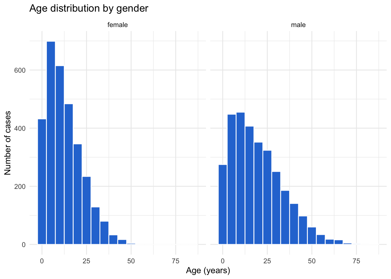
Note
facet_wrap(~ hospital_name, ncol = 2)sets the number of columnsfacet_wrap(~ hospital_name, scales = "free_y")lets each panel have its own y-axis (careful: it makes panels harder to compare)facet_grid(gender ~ outcome)makes a grid with one variable for rows and one for columns
Important✏️ TRY IT 6 (4 min): facets
Facet your measles epicurve by district (leave out “Unknown”). Did every district peak at the same time?
✅ Check: five panels; every district peaks in March
NoteShow solution
measles %>%
  filter(!is.na(report_date), district != "Unknown") %>%
  ggplot(mapping = aes(x = report_date, fill = vaccinated)) +
  geom_histogram(binwidth = 7, color = "white") +
  facet_wrap(~ district) +
  scale_fill_manual(values = vacc_colors) +
  scale_x_date(date_breaks = "2 months", date_labels = "%b") +
  labs(
    title = "Measles cases by week of report and district, 2024",
    x     = "Week of report",
    y     = "Number of cases",
    fill  = "Vaccinated"
  ) +
  theme_minimal()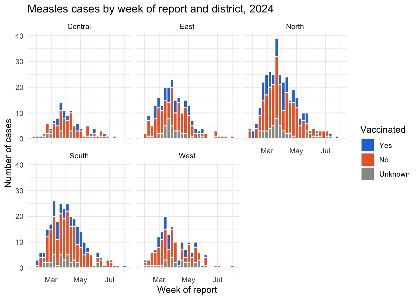
Roughly, yes: every district peaks in March, at about the same time as the overall outbreak. North has the most cases (its busiest week has 39).
Part 7: Saving plots
ggsave() saves the last plot you made, or a plot object you name. Save the plot as an object first:
👀 Follow along 7.1 — Save the epicurve as an object, then ggsave() it to outputs/epicurve.png (the next two code blocks).
epicurve <- linelist %>%
  filter(onset_date >= as.Date("2014-01-01")) %>%
  ggplot(mapping = aes(x = onset_date)) +
  geom_histogram(binwidth = 7, fill = "#2a78d6", color = "white") +
  labs(title = "Weekly cases", x = "Week of onset", y = "Number of cases") +
  theme_minimal()
Then save it to the outputs/ folder:
ggsave(here("outputs", "epicurve.png"), plot = epicurve,
       width = 8, height = 5, dpi = 300)
Tip⭐ Bonus
- Make a bar chart of the percentage of measles cases who died in each age group (
summarise()first, thengeom_col()). - Try
scale_fill_viridis_d()instead ofscale_fill_manual()on one of your plots. - Brought your own data? Make a bar chart, a plot over time (if you have dates), and a faceted plot, and save one of them with
ggsave().
See the solutions file for the code.
Extra: box plots with summary labels (optional)
This optional, advanced example calculates the median and quartiles for each group with summarise(), turns them into text, and adds them to the plot with geom_text() — combining Sessions 4, 5, and 6.
# 1. Summary statistics for each gender and outcome
box_stats <- linelist %>%
  filter(gender != "Unknown", outcome != "Unknown") %>%
  group_by(gender, outcome) %>%
  summarise(
    median = median(age_years, na.rm = TRUE),
    q1     = quantile(age_years, 0.25, na.rm = TRUE),
    q3     = quantile(age_years, 0.75, na.rm = TRUE),
    .groups = "drop"
  ) %>%
  mutate(label = paste0("Median: ", round(median, 1), "\n",
                        "Q1: ", round(q1, 1), "\n",
                        "Q3: ", round(q3, 1)))

# 2. The plot, with the labels placed beside each box
linelist %>%
  filter(gender != "Unknown", outcome != "Unknown") %>%
  ggplot(mapping = aes(x = gender, y = age_years)) +
  geom_boxplot(fill = "#2a78d6", alpha = 0.3, width = 0.35) +
  geom_text(
    data = box_stats,
    mapping = aes(x = gender, y = q3, label = label),
    nudge_x = 0.22, hjust = 0, vjust = 0, size = 2.8, color = "gray30"
  ) +
  facet_wrap(~ outcome) +
  scale_x_discrete(expand = expansion(add = c(0.4, 0.9))) +   # room on the right for the labels
  labs(
    title    = "Age distribution by gender and outcome",
    subtitle = "Labels show the median and quartiles",
    x        = "Gender",
    y        = "Age (years)"
  ) +
  theme_minimal()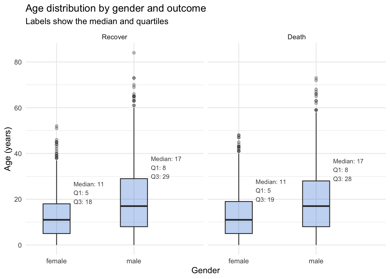
Key points
geom_bar()counts rows for you;geom_col()draws numbers you already calculated.- Order bars with
fct_infreq()/fct_reorder(), and use horizontal bars (aes(y = ...)) for long labels. position = "stack","fill"(100%, compares proportions), or"dodge"(side by side, compares counts).- Choose colors on purpose: colorblind-safe pairs (not red vs green), gray for “Unknown”, and a named color vector with
scale_fill_manual()so each category keeps its color. - An epicurve is a weekly histogram of a date column; format the axis with
scale_x_date(). Look at the whole date range first — plots reveal data errors. facet_wrap(~ COLUMN)makes small multiples with shared axes.- Save a plot as an object, then
ggsave(here("outputs", "file.png"), plot = ..., width, height, dpi).
Next: Session 8 — Programming (optional). Write your own functions, use if/else, and loop over groups — for example, to save one epidemic curve per hospital automatically.